
Usage of functions#
In this tutorial we compile examples on how to use the differnt functions available in the package. You can refer to previous tutorial to see how to use CellBender and perform quality control and basic downstream analysis of sc/snRNA-seq. We are going to use the object generated in the Quality control of sc/snRNA-seq.
Environment setup#
# Set-up
import anndata as ad
import dotools_py as do
import session_info


adata = ad.read_h5ad("/Users/david/Downloads/Data10x/adata.h5ad")
adata
2025-10-22 17:13:17,278 - Jupyter enviroment detected. Using "inline" backend
AnnData object with n_obs × n_vars = 2783 × 18517
    obs: 'batch', 'condition', 'n_genes_by_counts', 'log1p_n_genes_by_counts', 'total_counts', 'log1p_total_counts', 'total_counts_mt', 'log1p_total_counts_mt', 'pct_counts_mt', 'total_counts_ribo', 'log1p_total_counts_ribo', 'pct_counts_ribo', 'n_genes', 'n_counts', 'doublet_class', 'doublet_score', 'leiden', 'autoAnnot', 'celltypist_conf_score', 'annotation', 'annotation_recluster'
    var: 'highly_variable', 'means', 'dispersions', 'dispersions_norm', 'highly_variable_nbatches', 'highly_variable_intersection'
    uns: 'annotation_recluster_colors', 'hvg', 'leiden', 'log1p', 'neighbors', 'umap'
    obsm: 'X_CCA', 'X_pca', 'X_umap'
    layers: 'counts', 'logcounts'
    obsp: 'connectivities', 'distances'
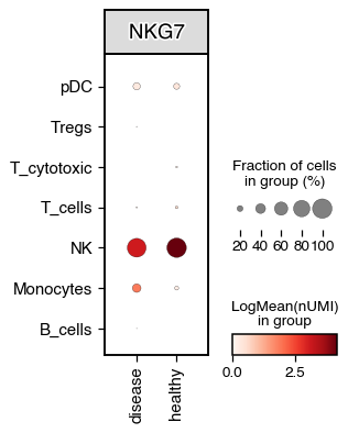
Dotplot#
The dotplot function builds on scanpy Dotplot method, but we also allow for the visualisation of 3 variables at the same time. For example, we can visualise the expression of a gene across celltypes and conditions
do.pl.dotplot(adata, x_axis="condition", features="NKG7", y_axis="annotation_recluster", figsize=(3, 4))
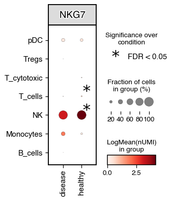
We can also perform differential testing between groups.
do.pl.dotplot(adata, x_axis="condition", features="NKG7", y_axis="annotation_recluster", figsize=(3, 4), add_stats="x_axis")
2025-10-22 16:45:41,616 - Error while testing: division by zero
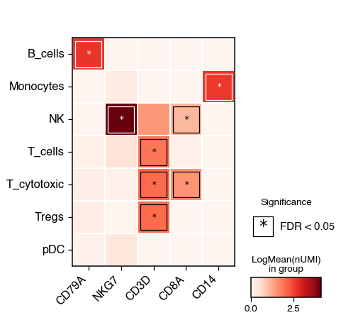
Heatmap#
The heatmap functions allow for the visualisation of the mean expression of genes across different groups. We can also test for significance and identify the group with the highest expression compared to the rest
do.pl.heatmap(
    adata,
    group_by="annotation_recluster",
    features=["CD79A", "NKG7", "CD3D", "CD8A", "CD14"],
    add_stats=True,
    xticks_rotation=45,
)
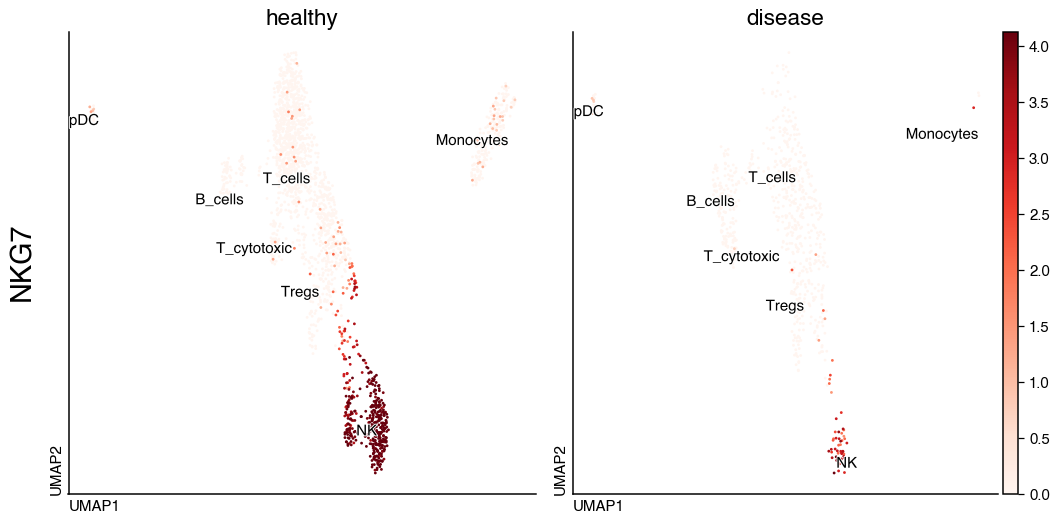
UMAP#
With do.pl.umap() we can visualise in UMAP embeddings the expression of genes as well as metadata information
do.pl.umap(adata, "NKG7", split_by="condition", share_legend=True, size=20, labels="annotation_recluster", figsize=(12, 6))
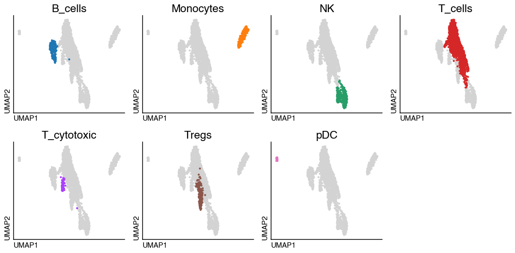
Split embeddings#
If we have categorical metadata we can visualise it also highlighting the different categories in each subplot
do.pl.split_embeddding(adata, split_by="annotation_recluster", ncols=4, figsize=(12, 6))
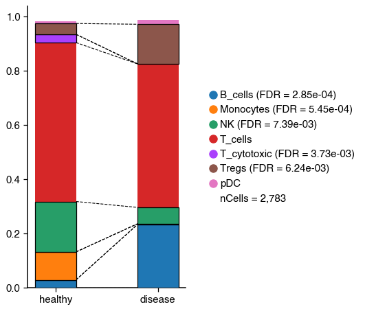
Changes in cell proportion#
As shown in the tutorial, we can also test for significant changes in cell population.
do.pl.cell_composition(
    adata, "annotation_recluster", "condition", "batch", condition_order=["healthy", "disease"], transform="arcsin"
)
[INFO] Your data doesn't have replicates! Artificial replicates will be simulated to run scanpro.
[INFO] Simulation may take some minutes...
[INFO] Generating 3 replicates and running 100 simulations...
[INFO] Finished 100 simulations in 1.09 seconds
2025-10-22 16:46:36,057 - There are 5 populations with a significant change
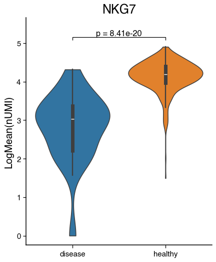
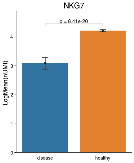
Expression of genes and continuous metadata#
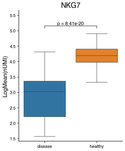
We can visualise the average expression of a gene in a celltype or continuous metadata information across condition with barplots, violinplots and boxplots. Additionally, we can test for significance.
nk = adata[adata.obs.annotation == "NK"]
do.pl.violinplot(nk, feature="NKG7", x_axis="condition", reference="healthy", groups="disease", figsize=(5, 6))
do.pl.barplot(nk, feature="NKG7", x_axis="condition", reference="healthy", groups="disease", figsize=(5, 6))
do.pl.boxplot(nk, feature="NKG7", x_axis="condition", reference="healthy", groups="disease", figsize=(5, 6))
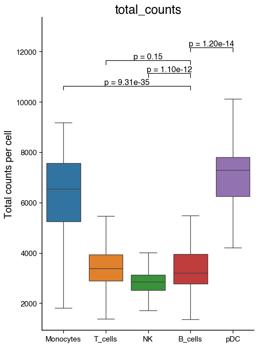
do.pl.boxplot(
    adata,
    "annotation",
    "total_counts",
    reference="B_cells",
    groups=["Monocytes", "NK", "T_cells", "pDC"],
    figsize=(6, 8),
    ylabel="Total counts per cell",
)
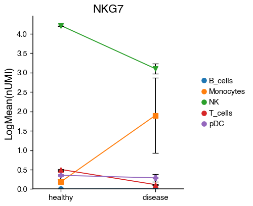
do.pl.lineplot(adata,
               x_axis="condition",
               features="NKG7",
               hue="annotation",
               xticks_order=["healthy", "disease"],
               )
{'mainplot_ax': <Axes: title={'center': 'NKG7'}, ylabel='LogMean(nUMI)'>,
 'legend_ax': <Axes: >}
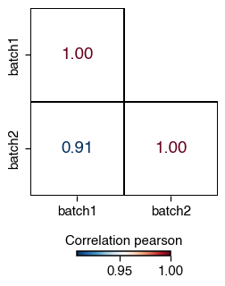
Correlation between condition#
We can also visualise the overall correlation between categorical metadata such as sample or condition.
do.pl.correlation(
    adata,
    group_by="batch",
    method="pearson",
    mask="upper",  # Hide the upper triangle
    mode="letters",  # alternative use colors
)
session_info.show(na=False, cpu=True, excludes=["backports"], std_lib=True, dependencies=True, html=True)
Click to view session information
-----
anndata             0.11.4
dotools_py          0.0.1
session_info        v1.0.1
sys                 3.10.16 (main, Dec 11 2024, 10:22:29) [Clang 14.0.6 ]
-----
Click to view modules imported as dependencies
Cython                      3.0.12
PIL                         11.2.1
adjustText                  1.3.0
appnope                     0.1.2
argparse                    1.1
arrow                       1.3.0
attr                        25.3.0
attrs                       25.3.0
babel                       2.16.0
bbknn                       1.6.0
brotli                      1.0.9
celltypist                  1.6.3
certifi                     2025.04.26
cffi                        1.17.1
chardet                     4.0.0
charset_normalizer          3.3.2
cloudpickle                 3.1.1
comm                        0.2.1
csv                         1.0
ctypes                      1.1.0
cycler                      0.12.1
cython                      3.0.12
dask                        2024.11.2
dateutil                    2.9.0.post0
debugpy                     1.8.11
decimal                     1.70
decorator                   5.1.1
defusedxml                  0.7.1
distutils                   3.10.16
doubletdetection            4.3
exceptiongroup              1.2.0
executing                   0.8.3
formulaic                   1.1.1
formulaic_contrasts         1.0.0
gseapy                      1.1.8
h5py                        3.13.0
idna                        3.7
igraph                      0.11.8
interface_meta              1.3.0
ipaddress                   1.0
ipykernel                   6.29.5
ipywidgets                  8.1.7
jedi                        0.19.2
jinja2                      3.1.6
joblib                      1.4.2
json                        2.0.9
json5                       0.9.25
jsonpointer                 2.1
jsonschema                  4.23.0
jupyter_events              0.12.0
jupyter_server              2.15.0
jupyterlab_server           2.27.3
kiwisolver                  1.4.8
leidenalg                   0.10.2
llvmlite                    0.44.0
logging                     0.5.1.2
markupsafe                  3.0.2
marshal                     4
matplotlib                  3.10.0
matplotlib_inline           0.1.6
more_itertools              10.3.0
msgpack                     1.1.0
natsort                     8.4.0
nbformat                    5.10.4
numba                       0.61.0
numcodecs                   0.13.1
numpy                       1.26.4
packaging                   24.2
pandas                      2.2.3
parso                       0.8.4
patsy                       1.0.1
phenograph                  1.5.7
platform                    1.0.8
platformdirs                4.3.7
pluggy                      1.5.0
polars                      1.30.0
prompt_toolkit              3.0.43
psutil                      5.9.0
pure_eval                   0.2.2
pyarrow                     19.0.1
pycparser                   2.21
pydeseq2                    0.5.1
pygments                    2.19.1
pynndescent                 0.5.13
pyparsing                   3.2.3
pytz                        2025.2
re                          2.2.1
requests                    2.32.3
rfc3339_validator           0.1.4
rfc3986_validator           0.1.1
scanpy                      1.11.1
scipy                       1.15.2
seaborn                     0.13.2
setuptools                  75.8.0
simplejson                  3.20.1
six                         1.17.0
sklearn                     1.5.2
sniffio                     1.3.0
socketserver                0.4
socks                       1.7.1
sparse                      0.16.0
sqlite3                     2.6.0
stack_data                  0.2.0
statsmodels                 0.14.4
stdlib_list                 0.11.1
tarfile                     0.9.0
tblib                       3.1.0
texttable                   1.7.0
threadpoolctl               3.6.0
tlz                         1.0.0
tomli                       2.0.1
toolz                       1.0.0
torch                       2.6.0
tornado                     6.5.1
tqdm                        4.67.1
traitlets                   5.14.3
umap                        0.5.7
urllib3                     2.3.0
wcwidth                     0.2.5
websocket                   1.8.0
wrapt                       1.17.2
yaml                        6.0.2
zarr                        2.18.3
zlib                        1.0
zmq                         26.2.0
zstandard                   0.23.0
-----
IPython             8.30.0
jupyter_client      8.6.3
jupyter_core        5.7.2
jupyterlab          4.3.4
notebook            7.3.2
-----
Python 3.10.16 (main, Dec 11 2024, 10:22:29) [Clang 14.0.6 ]
macOS-15.5-arm64-arm-64bit
10 logical CPU cores, arm
-----
Session information updated at 2025-07-08 17:11